| patient | time | trt | seizure | base | lbase |
|---|---|---|---|---|---|
| 1 | 1 | 0 | 5 | 11 | 2.3979 |
| 1 | 2 | 0 | 3 | 11 | 2.3979 |
| 1 | 3 | 0 | 3 | 11 | 2.3979 |
| 1 | 4 | 0 | 3 | 11 | 2.3979 |
| 2 | 1 | 0 | 3 | 11 | 2.3979 |
| 2 | 2 | 0 | 5 | 11 | 2.3979 |
| 2 | 3 | 0 | 3 | 11 | 2.3979 |
| 2 | 4 | 0 | 3 | 11 | 2.3979 |
ASR024. LMM with transformed response - Epilepsy treatment
The complete script for this example can be downloaded here:
Dataset
The models that we will fit here are based on the D020 dataset, and the first few rows are presented below:
Model
In this example, we will fit two identical LMMs. The first one using the raw response, and the second using log-transformed response. The specification of the model is:
\[ y = \mu + base + trt + time + trt:time + e\ \] where,\(y\) is the number of seizures,
\(\mu\) is the overall mean,
\(base\) is the fixed effect of the patient’s baseline number of seizures,
\(trt\) is the fixed effect of treatment,
\(time\) is the fixed effect of time of measurement,
\(trt:time\) is the fixed effect of the interaction between treatment and time of measurement,
\(e\) is the random residual effect, with \(e \sim \mathcal{N}(0,R)\).In the above model, the residual matrix \(\mathbf{R_i = I_m \otimes G}\) represents a direct product between a 4 \(\times\) 4 matrix (\(\mathbf{G}\)) describing the structure of each patient over their four time measurements. This implies a common variance for each time point and a common correlation between any time points. In addition, the second matrix (\(\mathbf{I_m}\)) is describing the independence between the \(m\) patients. We are considering \(\mathbf{R = \oplus R_i}\) to indicate that each level of trt will have its own estimates.
We will apply a logarithmic transformation on the response variable using:
where \(\,y_t\,\) is the transformed response variable.
Now, let’s take a look at how to write the models with ASReml-R. Note that before fitting them, trt, time, and patient need to be set as factors.
asr024 <- asreml(
  fixed = seizure ~ base + trt + time + trt:time,
  residual = ~dsum(~id(patient):corv(time)|trt),
  data = d020
)
In this model, we specified the residual structure to have, the error variance and a correlation between residual errors of each patient’s measurements. However, this structure is estimating different variance components for each of the treatment levels.
The same model is now fitted for the log-transformed response.
d020$trans <- log(d020$seizure + 1)asr024t <- asreml(
fixed = trans ~ base + trt + time + trt:time,
residual = ~dsum(~id(patient):corv(time)|trt),
data = d020
)Exploring output
Now, we can take a look at the distributions of the residuals for each model:
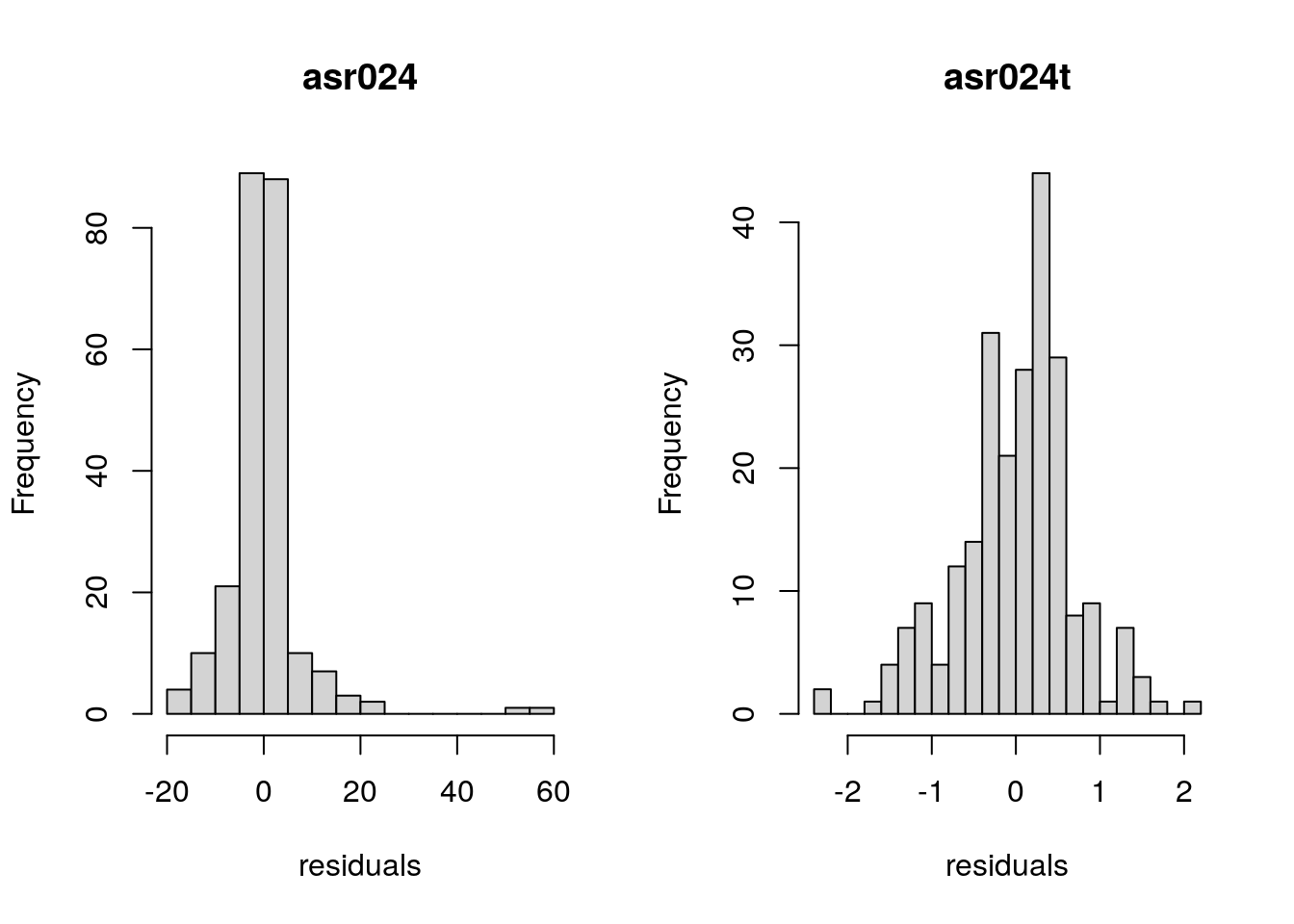
When looking at these histograms, we can see that with the transformed response variable, the distribution of the residuals looks to resemble ‘closer’ a Normal distribution compared to the model using raw responses. Hence, in this case, using the transformed data seems more appropriate.
Let’s take a look at the ANOVA table of the model with the log-transformed response:
wald(asr024, denDF = 'numeric')$Wald Df denDF F.inc Pr
(Intercept) 1 53.8 748.900 0.000000e+00
base 1 55.0 96.460 1.052491e-13
trt 1 55.5 3.158 8.104220e-02
time 3 168.9 1.514 2.126308e-01
trt:time 3 163.3 1.595 1.926594e-01Here we can see that the covariate base is the only significant model term (at a level of 5%).
The estimated variance components from this model are:
summary(asr024t)$varcomp component std.error z.ratio bound %ch
trt_0!R 1.0000000 NA NA F 0
trt_0!time!cor 0.2647827 0.10446757 2.534592 U 0
trt_0!time!var 0.4536678 0.06839227 6.633320 P 0
trt_1!R 1.0000000 NA NA F 0
trt_1!time!cor 0.4724659 0.09563289 4.940412 U 0
trt_1!time!var 0.5020254 0.08434048 5.952366 P 0Notice that, based on the z-ratios, the variance and correlation estimates seem to be significant. Also, it is easy to see some differences between the two treatment levels, particularly for the correlation estimates, with values of 0.26 and 0.47 for treatment levels \(0\) and \(1\), respectively.
The back transformation of the estimated number of seizures can be calculates using:
where \(\,y_{bt}\,\) is the back transformed estimation.
The predictions of the number of seizures per treatment, with back transformation, can be estimated with:
preds <- predict(asr024t, classify = 'trt')$pvals
preds <- as.data.frame(preds)
preds$back_trans <- exp(preds$predicted.value) - 1
trt predicted.value std.error status back_trans
1 0 1.868185 0.08526030 Estimable 5.476531
2 1 1.636085 0.09893421 Estimable 4.135027According to these results, the estimated numbers of seizures with the placebo and with the active treatment are 5.48 and 4.14, respectively.