ASReml-R Cookbook - ASR016. LMM for a split-split-plot design with a three-way factorial

Dataset

The model that we will fit here is based on the D013 dataset, and the first few rows are presented below:

rep	row	pos	spacing	stock	gen	yield	trt
R1	2	1	6	Seedling	Redspur	70.9	601
R1	2	2	6	Seedling	Golden	130.9	602
R1	2	8	6	MM111	Redspur	114.5	611
R1	2	7	6	MM111	Golden	90.5	612
R1	2	3	6	M0007	Redspur	151.8	671
R1	2	4	6	M0007	Golden	125.0	672
R1	2	5	6	MM106	Redspur	NA	661
R1	2	6	6	MM106	Golden	NA	662

Model

In this example we will fit a LMM for split-split-plot design. The specification of the model is: \[ y = \mu + spacing*stock*gen + rep + rep:wplot + rep:wplot:subplot + e\ \]

where,

\(y\) is the yield of apple,

\(\mu\) is the overall mean,

\(spacing\) is the fixed effect of the spacing between trees,

\(stock\) is the fixed effect of rootstock,

\(gen\) is the fixed effect of variety,

\(rep\) is the random effect of replicate (block),

\(rep:wplot\) is the nested random effect of spacing within rep, with \(rep:wplot \sim \mathcal{N}(0,\,\sigma^{2}_{w})\),

\(rep:wplot:subplot\) is the nested random effect of rootstock within spacing within rep, with \(rep:wplot:subplot \sim \mathcal{N}(0,\,\sigma^{2}_{s})\),

\(e\)

\(e \sim \mathcal{N}(0,\,\sigma^{2}_{e})\)

Note that before fitting the model with ASReml-R, the variables wplot and subplot need to be specified as they are not fully described in the data. This is because, in several instances, a level of spacing spanned across two rows. In such cases, this level of spacing need to be separated in two levels. Therefore wplot was defined as the concatenation of the factors row and spacing, and subplot was defined with the factors row, spacing and stock. Additionally, rep, spacing, stock, gen, wplot and subplot need to be set as factors.

d013 <- transform(d013, rep = factor(rep), spacing = factor(spacing), stock = factor(stock), gen = factor(gen),
                 wplot = factor(paste(row, spacing, sep = "_")),
                 subplot = factor(paste(row, spacing, stock, sep="_")))

Now, let’s take a look at how to write the model:

asr016 <- asreml(
  fixed = yield ~ spacing*stock*gen, 
  random = ~rep + rep:wplot + rep:wplot:subplot, 
  residual = ~units,
  data = d013
)

A relevant aspect is that the term spacing*stock*gen will be separated into its main effects, two-way interactions and the three-way interaction. In addition, one of the most important elements of this model is that the random effects of the above model define the hierarchical structure (multi-level) of this study.

Exploring output

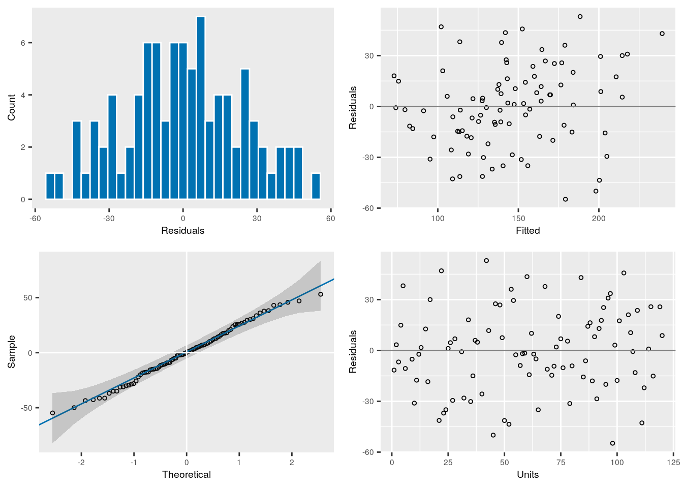
Here is how the residual diagnostic plots look like:

Let’s take a look at the incremental ANOVA table:

wald(asr016, denDF = 'numeric', ssType = 'incremental')$Wald


Wald tests for fixed effects.
Response: yield

                  Df denDF  F.inc      Pr
(Intercept)        1   3.9 337.10 0.00007
spacing            2   9.3   7.50 0.01145
stock              3  28.5   5.24 0.00528
gen                1  31.7   0.02 0.88155
spacing:stock      6  29.8   1.20 0.33490
spacing:gen        2  32.5   0.19 0.82773
stock:gen          3  32.0   6.19 0.00194
spacing:stock:gen  6  32.8   0.66 0.68124

Therefore, it might be of interest to report some estimated means for the significant model terms:

predict(asr016, classify = 'spacing')$pvals
predict(asr016, classify = 'stock:gen')$pvals

  spacing predicted.value std.error    status
1       6        122.1618  11.00745 Estimable
2      10        154.0613  10.99028 Estimable
3      14        166.5716  10.60588 Estimable

     stock     gen predicted.value std.error    status
1    M0007  Golden        161.9857  13.14218 Estimable
2    M0007 Redspur        139.6639  13.19385 Estimable
3    MM106  Golden        150.5247  13.85512 Estimable
4    MM106 Redspur        185.9478  12.14534 Estimable
5    MM111  Golden        120.1358  12.61858 Estimable
6    MM111 Redspur        144.2168  11.83218 Estimable
7 Seedling  Golden        155.8493  13.36959 Estimable
8 Seedling Redspur        122.4620  12.66707 Estimable

The variance components estimated from this model are:

summary(asr016)$varcomp

                  component std.error   z.ratio bound %ch
rep                197.4486  238.7933 0.8268599     P 0.1
rep:wplot          203.8158  244.4232 0.8338644     P 0.3
rep:wplot:subplot  193.3306  290.1201 0.6663812     P 0.3
units!R           1016.0373  288.6710 3.5197072     P 0.0